Packages and Data

Welcome to the workshop! On this page you’ll find information about the packages and data sets we’ll be using. The workshop proper starts on the Hello Arrow page, but you may find this page useful to read before the workshop begins.

Packages

To install the required packages, run the following:

install.packages(c(
  "arrow", "dplyr", "dbplyr", "duckdb", "fs", "janitor",
  "palmerpenguins", "remotes", "scales", "stringr", 
  "lubridate", "tictoc"
))

To load them:

library(arrow)
library(dplyr)
library(dbplyr)
library(duckdb)
library(stringr)
library(lubridate)
library(palmerpenguins)
library(tictoc)
library(scales)
library(janitor)
library(fs)

The workshop doesn’t use graphics or spatial data much but they are used on this page and again at the end. Suggested packages if you want to run those parts of the code can be installed with the following:

install.packages(c("ggplot2", "ggrepel", "sf"))

Load the packages with this:

library(ggplot2)
library(ggrepel)
library(sf)

Data

Throughout the workshop we’ll be relying on the New York City taxicab data set (instructions on obtaining the data are included below). In its full form, the data set takes the form of one very large table with about 1.7 billion rows and 24 columns. Each row corresponds to a single taxi ride sometime between 2009 and 2022. The contents of the columns are as follows:

vendor_name (string): A code indicating the service provider that maintains the taxicab technology system in that vehicle. Possible values here are “VTS”, “DDS” and “CMT”.
pickup_datetime (timestamp): Specifies the time at which the customer was picked up. This is stored as an Arrow timestamp, which is analogous to a POSIXct object in R and can be manipulated in similar ways.
dropoff_datetime (timestamp): Specifies the time at which the customer was dropped off.
passenger_count (int64): An integer specifying the number of passengers. Note that this is not automatically computed: the value is manually entered by the driver.
trip_distance (double): The elapsed trip distance reported by the taximeter. Note that this is a US based dataset so the distance is recorded in miles (not kilometers).
pickup_longitude (double): Longitude data for the pickup location
pickup_latitude (double): Latitude data for the pickup location
rate_code (string): Different trips charge fees at different rates, often due to airport surcharges, and those rates are assigned codes. String specifying the final rate code in effect at the end of the trip. Possible values are: “Standard rate”, “JFK”, “Newark”, “Negotiated”, “Nassau or Westchester”, and “Group ride”
store_and_fwd (string): Sometimes the vehicle does not have an internet connection and so the trip data is not immediately transmitted to the server. This is referred to as a “store and forward” case. The store_and_fwd flag is set to “Yes” when the vehicle did not immediately transmit, and “No” when it was able to transmit immediately.
dropoff_longitude (double): Longitude data for the dropoff location
dropoff_latitude (double): Latitude data for the dropoff location
payment_type (string): Variable indicating how the customer paid for the ride. Values that occur in the data are “Cash”, “Credit card”, “No charge”, “Dispute” and “Unknown” (and of course missing data), but “Voided trip” is also possible according to the original documentation.
fare_amount (double): The “time and distance” fare in US dollars calculated by the meter.
extra (double): Additional extras and surcharges added to the fare amount. This includes US$0.50 and US$1 rush hour and overnight charges.
mta_tax (double): The MTA is the “Metropolitan Transportation Authority” that governs public transport in New York City. This variable includes the US$0.50 MTA tax that is triggered based on the rate code in use.
tip_amount (double): In the US it is customary for passengers to provide the taxi driver with an additional “tip” payment for service. This field records the tip amount paid only for credit card transactions: cash tips are not recorded.
tolls_amount (double): As in many cities, various roads in NYC charge additional fees (“tolls”) to use them. Any tolls incurred are recorded here.
total_amount (double): This is the total amount charged to the customer (excluding cash tips, which are not recorded in the data set).
improvement_surcharge (double): The improvement surcharge is an additional US$0.30 fee that began in 2015. According to the official documentation it is “assessed on hailed trips at the flag drop”. I honestly have no idea what that means.
congestion_surcharge (double): As in many cities, NYC imposes a congestion surcharge for vehicles that enter certain locations in the city. Any congestion fee incurred is recorded here.
pickup_location_id (int64): The “TLC Taxi Zone” in which the pickup occurred. This is a numeric id ranging from 1 to 265: more information about the taxi zones is provided below.
dropoff_location_id (int64): The “TLC Taxi Zone” in which the dropoff occurred.
year (int32): The year in which the ride took place
month (int32): The month in which the ride took place

The tiny NYC taxi data set

In a moment we’ll talk about how to get the full data set, but let’s start with a simpler version!

In practice, not everyone has time or hard disk space to download the entire data set. On top of that, it’s not always a good idea to do your learning on an enormous data set: mistakes become more time consuming with big data. So it’s often helpful to practice with a smaller data set that has the exact same structure as the larger one that you want to use later. To help out with that, we’ve created the “Tiny NYC Taxi” data that contains only 1 in 1000 rows from the original data set. So instead of working with 1.7 billion rows of data and about 70GB of files, the tiny taxi data set is 1.7 million rows and about 80MB of files.

All you have to do is download the nyc-taxi-tiny.zip archive and unzip it, and you’re ready to start. On my machine I saved a copy of the data to a folder called "~/Datasets/nyc-taxi-tiny". So if I wanted to use the tiny taxi data for this workshop, I could open the data set with this command:

nyc_taxi <- open_dataset("~/Datasets/nyc-taxi-tiny")

The full NYC taxi data set

Obtaining a copy of the full data set requires a little bit more effort. It’s stored online in an Amazon S3 bucket, and you can download all the files directly from there. In fact, the arrow package has commands to do that. On my machine I saved the full data set to a folder called "~/Datasets/nyc-taxi", so the command I used looked like this:

copy_files(
  from = s3_bucket("ursa-labs-taxi-data-v2"),
  to = "~/Datasets/nyc-taxi"
)

Be warned!

Conceptually this is easy, but in practice it may be painful. Depending on the quality of your internet connection this is likely to take a long time. The data set is 69GB in size. The data set spans the years 2009 through 2022 and contains one parquet file per month. Here’s what you should expect to see for a single year:

list.files("~/Datasets/nyc-taxi/year=2018", recursive = TRUE)

 [1] "month=1/part-0.parquet"  "month=10/part-0.parquet"
 [3] "month=11/part-0.parquet" "month=12/part-0.parquet"
 [5] "month=2/part-0.parquet"  "month=3/part-0.parquet" 
 [7] "month=4/part-0.parquet"  "month=5/part-0.parquet" 
 [9] "month=6/part-0.parquet"  "month=7/part-0.parquet" 
[11] "month=8/part-0.parquet"  "month=9/part-0.parquet"

In any case, if you want to use the full NYC taxi data, the command you use to open the data set is the same: you just point R to the folder containing the full data set rather than the tiny one.

nyc_taxi <- open_dataset("~/Datasets/nyc-taxi/")

Regardless of which version of the data you’re using, you’re good to go.

Ancillary data files

Before moving on, it’s worth mentioning that the NYC taxi data website also includes a taxi_zone_lookup.csv file that includes human-readable names for the taxi zones. We’ll be using that file in the workshop, so you may wish to download iit also. Here’s a quick look at its contents:

zones <- read_csv_arrow("data/taxi_zone_lookup.csv")
zones

# A tibble: 265 × 4
   LocationID Borough       Zone                    service_zone
        <int> <chr>         <chr>                   <chr>       
 1          1 EWR           Newark Airport          EWR         
 2          2 Queens        Jamaica Bay             Boro Zone   
 3          3 Bronx         Allerton/Pelham Gardens Boro Zone   
 4          4 Manhattan     Alphabet City           Yellow Zone 
 5          5 Staten Island Arden Heights           Boro Zone   
 6          6 Staten Island Arrochar/Fort Wadsworth Boro Zone   
 7          7 Queens        Astoria                 Boro Zone   
 8          8 Queens        Astoria Park            Boro Zone   
 9          9 Queens        Auburndale              Boro Zone   
10         10 Queens        Baisley Park            Boro Zone   
# … with 255 more rows

Finally, it’s also worth mentioning that the website has a shapefile specifying the boundaries of the taxi zones and a csv file with some additional information about them. The tutorial doesn’t use this spatial data (except very briefly at the very end) so you ton’t really need it, but it’s helpful to mention here because it’s a hany way to make sense of the geography of the taxi zones. Using the shapefile together with the sf and ggplot2 packages we can draw a map of the taxi zones coloured by their numeric identifier:

shapefile <- "data/taxi_zones/taxi_zones.shp"
shapedata <- read_sf(shapefile)

shapedata |> 
  ggplot(aes(fill = LocationID)) + 
  geom_sf(size = .1) + 
  theme_bw() + 
  theme(panel.grid = element_blank())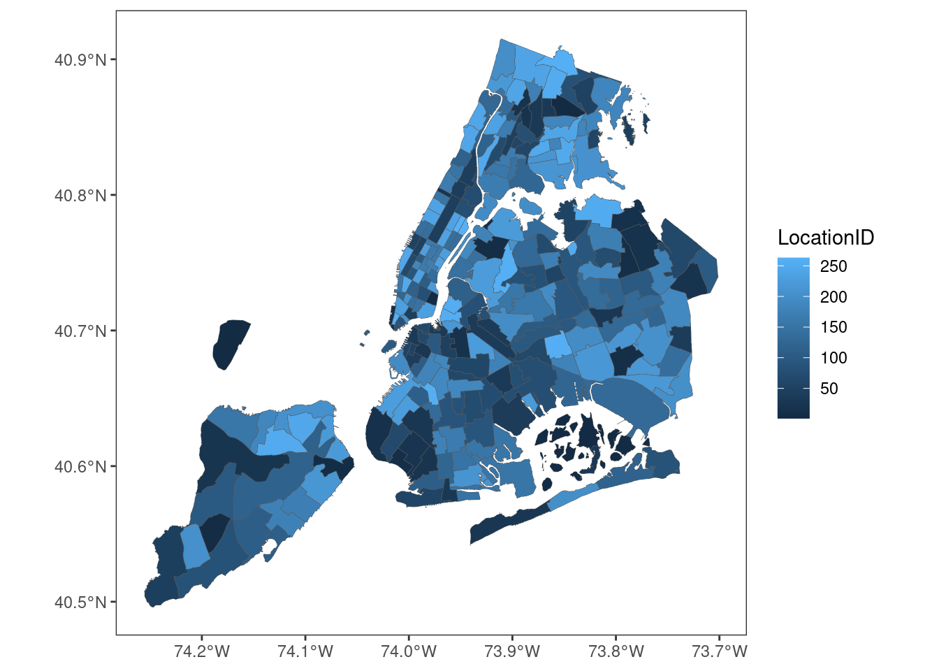

It’s not really needed, but if you do want a copy of this shapefile, download and unzip the taxi_zones.zip archive file.

Checks

Loading the data

Here’s what you should expect to see when you print the nyc_taxi object:

nyc_taxi

FileSystemDataset with 158 Parquet files
vendor_name: string
pickup_datetime: timestamp[ms]
dropoff_datetime: timestamp[ms]
passenger_count: int64
trip_distance: double
pickup_longitude: double
pickup_latitude: double
rate_code: string
store_and_fwd: string
dropoff_longitude: double
dropoff_latitude: double
payment_type: string
fare_amount: double
extra: double
mta_tax: double
tip_amount: double
tolls_amount: double
total_amount: double
improvement_surcharge: double
congestion_surcharge: double
pickup_location_id: int64
dropoff_location_id: int64
year: int32
month: int32

Okay, so we’re nyc_taxi linked to 158 files. What does that mean in terms of number of rows? How big is the table?

nrow(nyc_taxi)

[1] 1672590319

About 1.7 billion rows. That’s quite a lot.

A dplyr pipeline

If you want to make sure everything is working properly, let’s do a simple analysis. We’ll count the number of trips with destinations in each zone:

zone_counts <- nyc_taxi |> 
  count(dropoff_location_id) |> 
  arrange(desc(n)) |> 
  collect() 

zone_counts

# A tibble: 265 × 2
   dropoff_location_id          n
                 <int>      <int>
 1                  NA 1249152360
 2                 236   16489001
 3                 161   15643391
 4                 237   15526930
 5                 170   13328885
 6                 162   12631075
 7                 230   12565352
 8                  48   11482627
 9                 234   11276120
10                 142   11136863
# … with 255 more rows

In order for this to calculation to work, both arrow and dplyr need to be installed and loaded, so this pipeline should work as a good test to see if your installation is working properly!

Extras!

A few other things just for interests sake. If you’re curious to know how long the analysis is expected to take, this is how long it took to run on my laptop. For the sake of simplicity, throughout the workshop we’ll use the tictoc package for timing:

tic() # start timer
nyc_taxi |> 
  count(dropoff_location_id) |> 
  arrange(desc(n)) |> 
  collect() |> 
  invisible() # suppress printing
toc() # stop timer

37.541 sec elapsed

To give a sense of what this result means geographically, because the zones codes aren’t very meaningful without seeing them on a map, here’s that result shown as a heat map:

left_join(
  x = shapedata, 
  y = zone_counts, 
  by = c("LocationID" = "dropoff_location_id")
) |> 
  ggplot(aes(fill = n)) + 
  geom_sf(size = .1) + 
  scale_fill_distiller(
    name = "Number of trips",
    limits = c(0, 17000000), 
    labels = label_comma(),
    direction = 1
  ) + 
  theme_bw() + 
  theme(panel.grid = element_blank())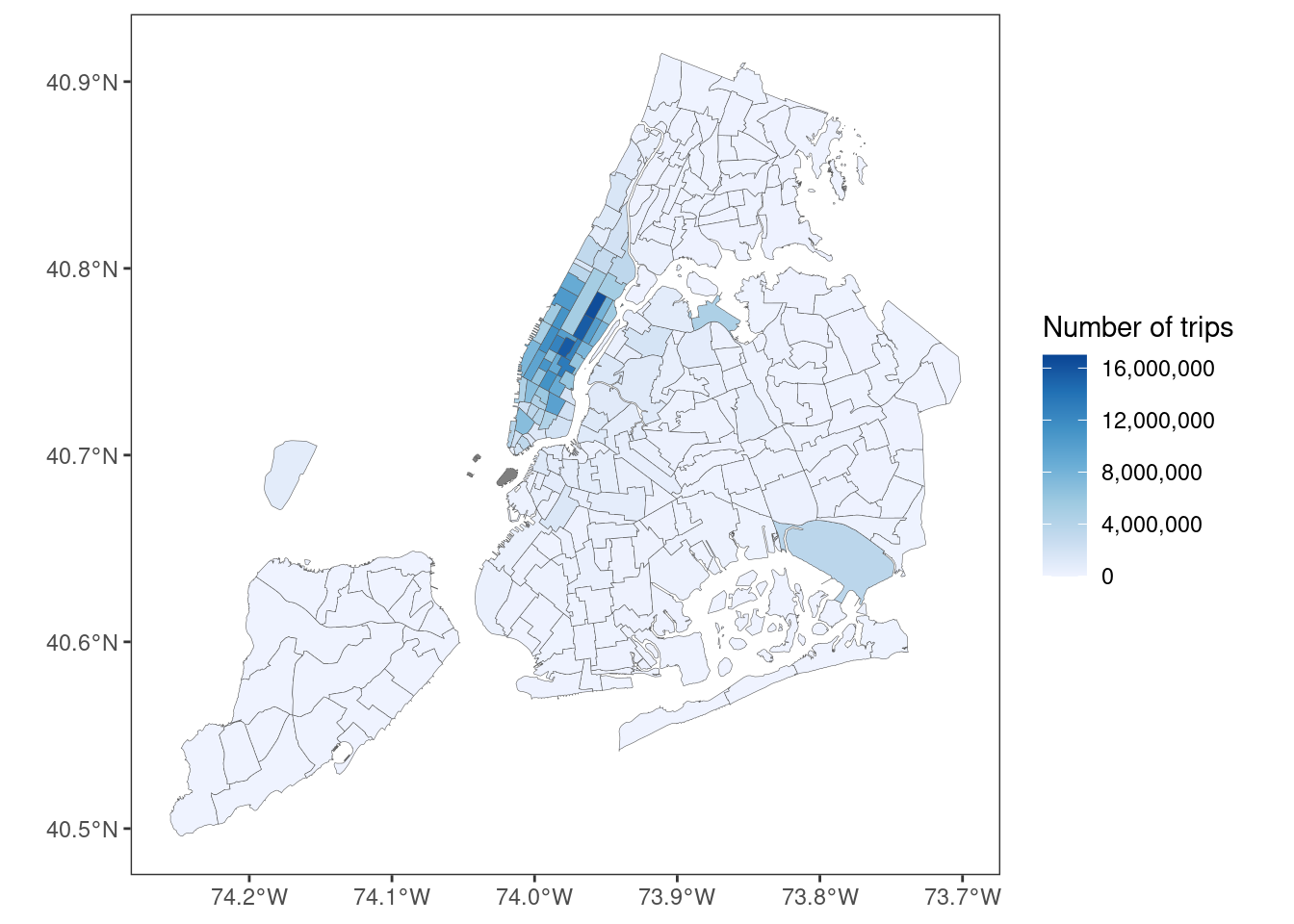

Pretty, yes?